A. Procedure : single subject
B. Source code: spm_realign.m
C. Notes

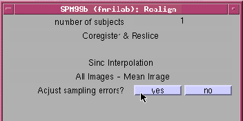
•number of subjects: 1

•num sessions for subject 1: 2

- scans for sunject1, secc1: afmri_r10010.img~afmri_r10011.img (done)

- scans for sunject1, secc2: afmri_r10012.img~afmri_r10013.img (done)

•Which option?...

- Coregister only

- Reslice only

- *Coregister & reslice <x>

•Reslice interpolation method?...

- Trilinear Interpolation

- *Sinc Interpolation <x>

- Fourier space interpolation

•Create what?...

- All images (1..n)

- Images 2..n

- * All Images + Mean Image <x>

- Mean Image Only

•Adjust sampling errors? yes <x> no

Realign: working on subject

B.1 function spm_realign(arg1,arg2,arg3,arg4,arg5,arg6)

1. This routine realigns a time-series of images acquired from the same subject using a least squares approach and a 6 parameter (rigid body) spatial transformation. The first image in the list specified by the user is used as a reference to which all subsequent cans are realigned. The reference scan does not have to the the first chronologically and it may be wise to chose a 'representative scan' in this role.
2. For fMRI data an additional adjustment is made to the data that removes a tiny amount of the movement-related confounds of these effects. However, it may be preferable to include the functions of the estimated movement parameters as confounds in the statistics part.

3. Uses :
Primarily to remove movement artefact in fMRI and PET time-series (or more generally longitudinal studies)

4. Inputs:
A series of *.img conforming to SPM data format (see 'Data Format'). The relative displacement of the images should be small with respect to their resolution. This is usually easy to ensure for functional images (e.g. fMRI, PET SPECT).

5. Outputs:

The parameter estimation part writes out ".mat" files for each of the input images. The part of the routine that writes the resliced images uses information in these ".mat" files and writes the realigned *.img files to the same subdirectory prefixed with an 'r' (i.e. r*.img). The details of the transformation are displayed in the results window as plots of translation and rotation. A set of realignment parameters are saved for each session, named: realignment_params_*.txt.

6. The Prompts Explained ---

% 'number of subjects'

Enter the number of subjects you wish to realign. For fMRI, it will ask you the
number of sessions for each subject. In the coregistration step, the sessions are
first realigned to each other, by aligning the first scan from each session to the
first scan of the first session. Then the images within each session are aligned to
the first image of the session. The parameter estimation is performed this way
because it is assumed (rightly or not) that there may be systematic differences in
the images between sessions. The adjustment step (correcting for resampling
artifacts) is also performed completely independantly between each of the fMRI
sessions.

% 'select scans for subject ..'

Select the scans you wish to realign. All operations are relative to the first image
selected.

==== Note that not all of the following prompts may be used ====

% 'Which option?'

- 'Coregister only'

Only determine the parameters required to transform each of the images 2..n to
the same space as image 1. The determined parameters for image XXXX.img are
saved in the file XXXX.mat. This is a Matlab file, containing the matrix 'M'. The
location of an image voxel (in mm) can be determined by computing
(1:3,:)*[xcoord ycoord zcoord 1]. Note that if the coregistration is performed
more than once on the unresliced data, the starting estimates are obtained from
parameters stored in the '.mat' files. Note that for PET, the coregistration is a two
step process.First of all, the ages are all realigned to the first in the series. A
mean of these realigned images is created, and a second pass realignment is
performed to realign all the images to the mean. Finally, the parameters are
corrected for any differences estimated by registering the first image in the series to the mean image.

- 'Reslice Only'

Reslice the specified images according to the contents of the previously
determined parameters. The images are resliced to be in the same space as
the first one selected. For fMRI, this is the first image of the first session.

- ‘Coregister & Reslice'

Combine the above two steps together.

Options for reslicing:

% 'Create what?'

- 'All Images (1..n)'

This reslices all the images - including the first image selected- which will
remain in it's original position.

- 'Images 2..n'

Reslices images 2..n only. Useful for if you wish to reslice (for example) a
PET image to fit a structural MRI, without creating a second identical MRI
volume.

- 'All Images + Mean Image'

In addition to reslicing the images, it also creates a mean of the resliced image.

- 'Mean Image Only'

Creates the mean image only.

% 'Mask the images?'

To avoid artifactual movement-related variance. Because of subject motion, different images are likely to have different patterns of zeros from where it was not possible to sample data. With masking enabled, the program searches through the whole time series looking for voxels which need to be sampled from outside the original images. Where this occurs, that voxel is set to zero for the whole set of images (unless the image format can represent NaN, in which case NaNs are used where possible).

% 'Adjust sampling errors?' (fMRI only)

Adjust the data (fMRI) to remove interpolation errors arising from the reslicing of the data. The adjustment for each fMRI session is performed independantly of any other session. Bayesian statistics are used to attempt to regularize the adjustment in order to prevent an excessive amount of signal from being removed. A priori variances for coefficients are assumed to be stationary and are estimated by translating the first image by a number of different distances using both Fourier and sinc interpolation. This gives a ball park figure on how much error is likely to arise because of the approximations in the sinc interpolation. The certainty of the solution is obtained from the residuals after fitting the optimum linear combination of the basis functions through the data. Estimates of certainty based on the residuals are unfortunately just an approximation. We still don't fully understand the nature of the movement artifacts that arise using fMRI. The current model is simply attempting to remove interpolation errors. There are many other sources of error that the model does not attempt to remove. It is possible that adjusting the data without taking into account the design matrix for the statistics may be problematic when there are stimulous correlated movements, since adjusting seperately requires the assumption that the movements are independant from the paradigm. It MAY BE BE BETTER TO INCLUDE THE ESTIMATED MOTION PARAMETERS AS CONFOUNDS WHEN THE STATISTICS ARE RUN. The motion parameters are saved for each session, so this should be easily possible.

% 'Reslice Interpolation Method?'

- 'Trilinear Interpolation'
Use trilinear interpolation (first-order hold) to sample the images during the
writing of realigned images.

- 'Sinc Interpolation'

Use a sinc interpolation to sample the images during the writing of realigned
images. This is slower than bilinear interpolation, but produces better results.
It is especially recommended for fMRI time series. An 9x9x9 kernel is used to
resample the images.

- 'Fourier space Interpolation' (fMRI only)

Rigid body rotations are executed as a series of shears, which are performed in
Fourier space (Eddy et. al. 1996). This routine only supports cubic voxels
(since zooms can not be done by convolution in Fourier space).

7. The `.mat' files.

This simply contains a 4x4 affine transformation matrix in a variable `M'. These files are normally generated by the `realignment' and `coregistration' modules. What these matrixes contain is a mapping from the voxel coordinates (x0,y0,z0) (where the first voxel is at coordinate (1,1,1)), to coordinates in millimeters (x1,y1,z1). By default, the the new coordinate system is derived from the `origin' and `vox' fields of the image header.

x1 = M(1,1)*x0 + M(1,2)*y0 + M(1,3)*z0 + M(1,4)

y1 = M(2,1)*x0 + M(2,2)*y0 + M(2,3)*z0 + M(2,4)

z1 = M(3,1)*x0 + M(3,2)*y0 + M(3,3)*z0 + M(3,4)

Assuming that image1 has a transformation matrix M1, and image2 has a

transformation matrix M2, the mapping from image1 to image2 is: M2\M1

(ie. from the coordinate system of image1 into millimeters, followed by a mapping from millimeters into the space of image2). These `.mat' files allow several realignment or coregistration steps to be combined into a single operation (without the necessity of resampling the images several times). The `.mat' files are also used by the spatial normalisation module.

B.2 function reslice_images(P,Flags,sessions)

% FORMAT reslice_images(P,Flags,sessions)

P - matrix of filenames {one string per row}

All operations are performed relative to the first image.

ie. Coregistration is to the first image, and resampling

of images is into the space of the first image.

sessions - the last scan in each of the sessions. For example,

the images in the second session would be

P((sessions(2-1)+1):sessions(2),:).

Flags - options flags

c - adjust the data (fMRI) to remove movement-related components.

k - mask output images

To avoid artifactual movement-related variance the realigned

set of images can be internally masked, within the set (i.e.

if any image has a zero value at a voxel than all images have

zero values at that voxel). Zero values occur when regions

'outside' the image are moved 'inside' the image during

realignment.

i - write mean image

The average of all the realigned scans is written to

mean*.img.

S - use sinc interpolation for reslicing (9x9x9).

n - don't reslice the first image

The first image is not actually moved, so it may not be

necessary to resample it.

N - don't reslice any of the images - except possibly create a

mean image.

a - write absolute values in images - more appropriate for fMRI.

The spatially realigned and adjusted images are written to

the orginal subdirectory with the same filename but prefixed
with a 'r'. They are all aligned with the first.

B.3 function realign_images(P,Q,sessions)

%FORMAT realign_images(P,Q,sessions)

P - matrix of filenames {one string per row}

All operations are performed relative to the first image.

ie. Coregistration is to the first image, and resampling

of images is into the space of the first image.

sessions - the last scan in each of the sessions. For example,

the images in the second session would be

P((sessions(2-1)+1):sessions(2),:).

Q - an optional matrix of filenames. These are used for masking

out regions which are (roughly) considered to be outside the

brain. The last filename is an image containing values

between zero and one, where each value is a weight. The

other images are template images. The way that this works is

that the first image in the series is matched (using an affine

transformation) to a linear combinantion of the template images.

This affine mapping can then be used to overlay the weight image

over the first image of the series.

B.4 function reslice_images_volbyvol(P,Flags,sessions)

% Reslices images volume by volume

% FORMAT reslice_images_volbyvol(P,Flags,sessions)

P - matrix of filenames {one string per row}

All operations are performed relative to the first image.

ie. Coregistration is to the first image, and resampling

of images is into the space of the first image.

sessions - the last scan in each of the sessions. For example,

the images in the second session would be

P((sessions(2-1)+1):sessions(2),:).

Flags - options flags

k - mask output images

To avoid artifactual movement-related variance the realigned

set of images can be internally masked, within the set (i.e.

if any image has a zero value at a voxel than all images have

zero values at that voxel). Zero values occur when regions

'outside' the image are moved 'inside' the image during

realignment.

i - write mean image

The average of all the realigned scans is written to

mean*.img.

S - use sinc interpolation for reslicing (9x9x9).

n - don't reslice the first image

The first image is not actually moved, so it may not be

necessary to resample it.

N - don't reslice any of the images - except possibly create a

mean image.

The spatially realigned images are written to the orginal

subdirectory with the same filename but prefixed with an 'r'.

They are all aligned with the first.

The only reason for reslicing a series plane by plane is to do the adjustment.

C. Notes

1. New features of Realign in SPM99

- handles multiple fMRI sessions

- two pass procedure for PET realignment (images registered to mean)

- checks for stopping criterion

- Fourier interpolation (for data with isotropic voxels)

- algorithm generally improved

- saves realignment parameters for use as confounds to stats

2. A number of modifications have been made to the realignment module. Many of these reflect the questions asked on the SPM discussion list. The realignment can be thought of as three components: parameter estimation, image resampling and correction of motion artifacts (adjustment).
3. fMRI sessions are now handled differently, because of the assumption that there may be systematic differences between the images in different sessions. The first volume of each session is now aligned to the first volume of the first session. Subsequent volumes in each session are then aligned to the first volume of the session. This should acheive increased accuracy within session, since all the images are aligned to an image from the same session. This also saves time, because subject movement between sessions tends to be larger than subject movement within session. The large systematic differences between sessions are therefore removed in the first realignment step. Adjustment is performed separately for each session, but the same mask for writing the realigned images is used for all images of all sessions.
4. PET realignment is now a two pass procedure. The first pass aligns all the images to the first image in the series. A mean of the realigned images is created, and the second pass aligns all the images to the mean. The second pass effectively matches the images to a less noisy template, and so should result in more accurate movement estimates.
5. Previously, the estimates of motion continued for a fixed number of iterations. This may be OK for small movements, but was inadequate for large ones. The realignment now continues until a stopping criterion has been achieved.
6. Movement estimation begins by using (faster but less accurate) tri-linear interpolation to resample the data. The final iterations are done using sinc interpolation in order to obtain the final high accuracy.
7. The algorithm for the SPM96 motion correction was very similar to that of the previous version (SPM94). However, both these implementations included an assumption about the rate of change of sum of squared difference with respect to parameter changes that only held when the rotations were small. This has been fixed.
8. Occasionally it may be necessary to attempt to sample voxels that lie outside the field of view of the original image. The parameter estimates in the SPM96 implementation assumed that the values of such voxels should be zero. In SPM99, these voxels are excluded from the computation of motion estimates.
9. The sinc interpolation has changed. In the previous version, the width of the hanning window was 1 pixel narrower than the optimal width. This has been fixed. Also, the integral under the sinc kernal has been set to one (by a renormalizing step). Both odd and even numbers of neighbours can now be used by the interpolation. Windowed sinc interpolation schemes are acheived by passing a negative hold to functions such as spm_sample_vol. Positive holds will result in polynomial (Lagrange) interpolation being used, whereas negative holds use sinc interpolation. The gradient of the images can also be directly obtained by spm_sample_vol.
10. A three dimensional Fourier interpolation has been implemented that is based on the paper by Eddy et al. This method is used for resampling fMRI data, but it requires the voxel sizes of the images to all be isotropic (since zooming can not be performed using this method). Preliminary tests showed that this method did not greatly reduce the resampling errors.
11. The fMRI adjustment has been modified. Rather than removing signal that is correlated to functions of the six parameters describing the rigid body movement of the subject, the adjustment now uses functions that are dependant upon the displacement of each voxel. This requires three parameters to describe it rather than six, but it is now a different function for each voxel. The functions that are covaried from the data are periodic in terms of the number of voxels displaced, and are based upon sines and cosines of the number of voxels displaced. e.g., the functions for a displacement of two voxels are identical to the functions for a displacement of one voxel. The functions were appropriate for simulated data, and with phantom data that was "moved" by moving the field of view of the scanner. However, the method is not quite so good for real subject movement within the scanner.
12. The adjustment step is now regularized. This regularization is based upon Bayesian statistics which states that: p(a|b) \propto p(b|a) \times p(a) . If (a) is the coefficients of the regressors, and (b) is the data, we wish to find the suitable values for (a) which maximize the posteriori probability of (a) given (b). Taking the Gibb's transform of these functions gives us:

       H(a|b) = H(b|a) + H(a) + c
which expresses the Bayesian furmulation in terms of energy cost functions. The objective is now to find the coefficients that minimize the cost function. The model assumes that the errors on (b) are normally distributed, and that H(b|a) is proportional to the residual sum of squares between the data and the fitted function. Probability

distributions for H(a) are estimated by translating the first image of the series by different amounts, using the windowed sinc function, and Fourier interpolation. This allows an estimate to be made for the a priori distribution of the errors.